Cybersecurity problem solving with explainable machine learning
Disclaimer: Nothing in this blog is related to the author’s day-to-day work. The content is neither affiliated nor sponsored by any companies.
Have you ever wondered why the model’s performance degrades after two months of initial deployment? Why does the model continue to make errors on certain samples? Why do bad cases from the operations team take so long to resolve? Such many ‘whys’ remind us that, explainable machine learning, which provides a way for human to understand what the model is doing on a given sample may be useful for cybersecurity problem solving.
The explainable model prediction is closely related to operations when solving cybersecurity problems. For example, firewall products must have sufficient confidence in the prediction results to block threats, and SIEM and SOAR systems on the cloud must introduce specific reasons and contextual associations of prediction results to support operational judgments. We can provide partial explainability of the prediction results to support operations based on the model’s explainability.
Explainable artificial intelligence (XAI) and its subfield, explainable machine learning, have been studied from a variety of perspectives in academia. This post introduces the black-box explainable model and some of its methods and applications in industry, as well as its design, usage, and limitations, among other things. My dear readers can delve deeper into this research topic by using the example of encrypted traffic detection, which causes the most headaches in cybersecurity.
Feel the vibe of explainable machine learning
In the cybersecurity industry, there are many machine learning models based on statistical features for network traffic detection and classification, such as the packet feature based detection model for encrypted DNS (DoH), mentioned in my previous post (and the Jupyter Notebook). These “counting” features are sliced to branch out the decision tree in boosting learner like xgboost, but the slicing strategy is decided by the learner, so the finer the slicing, the greater the risk of generalization to unknown data. The degradation of model performance and the instability of features from data drift needs continuous investment in maintenance by the data scientist team and even causes the data team to avoid solving traffic detection problems. Here, explainable machine learning can effectively solve such headaches.
It is worth mentioning here about the existing best practice of such encrypted traffic classification problems in computational advertisement using
GBDTcross features. He et al “Practical Lessons from Predicting Clicks on Ads at Facebook”*divides the counting features into sparse vectors and solves them with a simple linear model, which controls the slicing of statistical features to some extent; there are also cases where raw network traffic data is fed directly to a deep convolutional neural network to extract features; however, the neural network does not guarantee a reasonable extraction of encrypted traffic features and sufficient generalization, and the same design of fully connected layers for classification as in the computer vision problem doesn’t always outperform the tree learner.
To solve this problem, we employ the SHAP (SHapley Additive exPlanations) algorithm *. SHAP addresses the economics of cooperative competition from a game theory point of view: how to fairly measure A B C’s contribution to the $1,000 prize they receive by cooperating with one another? In this context, “fair measurement” takes into account three people’s independent contributions, two people’s cooperation (including the sequence), three people’s cooperation, and the relationship between two people’s cooperation and three people’s cooperation. The SHAP algorithm analogizes the model’s input features to cooperative individuals, and its interpretable contribution values are derived from the Nobel Prize-winning economics method Shapley value*. Because of the various combinations of contributors (feature vectors) that must be considered in the actual computation, the computational complexity of the exact solution is NP hard. The SHAP algorithm approximates the results in effective time using linear constraints, please feel free to find this interesting paper in the references.
In practice, the open source implementation of SHAP has been optimized for various types of prediction models, such as Tree SHAP for decision tree models. By simply adding these lines of code, the xgboost model for detecting encrypted DNS can use SHAP to interpret its prediction results:
import shap
explainer = shap.Explainer(clf.best_estimator_)
shap_values = explainer(train[features])

# visualize the first prediction's explanation
shap.plots.waterfall(shap_values[0])
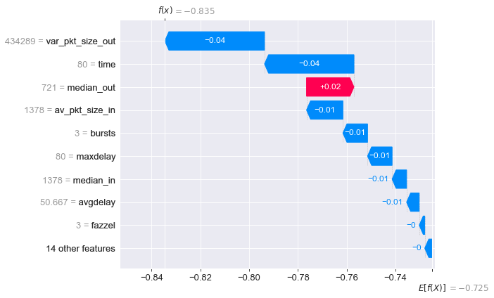
The figure of waterfall of SHAP values above shows that the expected value for all samples in the dataset is -0.725, while the model predicts -0.835 for sample 0. It’s because features like var_pkt_size_out and time push it from -0.725 to -0.835, while median_out feature pulls it back to the expectation of all samples. With back-n-forth pulling forces, the model eventually predicts -0.835 for sample #0 and correctly predicts it as a negative sample (non-encrypted DNS).
For positive sample #33 (encrypted DNS), median_out and median_in contribute significantly to its deviation from the expectation of all samples, lowering its prediction to -0.187 in a single kick and correctly predicting it as a positive sample.
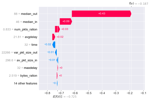
The two features median_out and median_in are also important in distinguishing the majority of positive samples in this dataset, and var_pkt_size_out is dominating in distinguishing negative samples. This explanation serves as the foundation for the decision to use the model approach: the model must be deployed with strict monitoring of the adversarial attack against these three features, for example:
- Whether there is a new encrypted DNS service that obfuscates the
median_outandmedian_instatistical features to escape from detection. - Whether the design data collection scenario includes a selection bias for features like
var_pkt_size_out - Whether these determining features have a consistent statistical distribution across data collected at different time periods
where “change in the statistical distribution of the determining features” is one of the primary causes of performance degradation after deployment and go-online. It is a type of data drift, and finding these features and monitoring their distribution can help detect and deal with it in real time. You can continue to investigate other SHAP functions, such as force_plot to better understand the basis of model classification. Of course, one can view the SHAP waterfall plot for each sample in the Jupyter Notebook, and one can also change the parameters of the prediction model to see how the SHAP waterfall plot changes with the new parameters.
The SHAP example demonstrates a general approach to the use of black-box explainable machine learning models, which essentially have the following properties:
- The modeling process requires developing a predictive model and then using another model to explain it, known as “post hoc” (explanation after the fact);
- The explainable model always provides the explanation but is unconcerned about the prediction method or whether the results are correct or not;
- The explainable model generates a waterfall plot of SHAP values for each sample rather than an overall explanation of the data set.
Similar to SHAP, there are other methods such as LIME * that explain the classifer model in a post-hoc black box. One can refer to the book “Interpretable Machine Learning”* for further study.
With feature importance, do we still need explainable models?
What is the difference between the SHAP value and the permutation feature importance? The SHAP value of each feature is related to each sample, describing the marginal effect of the combination of features in classification for the specific sample, and the combination of features and their marginal effect may differ for positive and negative samples, whereas the feature importance describes the model’s overall understanding of the whole dataset, describing the model classification performance for the dataset, independent of any specific samples. We can use the distribution of SHAP values on different samples to improve model characteristics, and Kaggle competitors can also optimally adjust the competition model by understanding the distribution of SHAP values *. Please refer to SHAP Summary Plot and Dependence Plot.
Of course, SHAP is not the only approach. There are numerous alternatives on the path to explainable machine learning and XAI.
Some models are inherently interpretable, such as symbol-based AI models * such as logical reasoning, the results of which can be self-explanatory. My previous post has mentioned my team’s work “Honeypot + graph learning + reasoning = scale up your emerging threat analysis” in which a knowledge graph model uses logical reasoning to explain the results of the distributed embedding model. The results of logistic regression and linear regression are also represented by a single weight matrix that is self-explanatory; the results of kNN models are also self-explanatory.
Explainable models are further subdivided into generic models such as SHAP and LIME, as well as some scenario-specific models such as the attention mechanism, which can provide some explanation for the results of transformer families such as BERT/GPT, as recently demonstrated by Deepmind’s AlphaCode in its demo*. Some adversarial generative models (GANs) generate adversarial samples in order to confuse model classification and, to some extent, reveal potential flaws or implicit assumptions in models.
Please read and explore “Explainable AI Cheat Sheet”* listed in the references for a good overview of existing explainable AI (XAI) models.
Keep calm and we still need other work
I kind of agree that, Please Stop Doing “Explainable” ML !* Because…
Explainable models have a natural limitation: their scope is limited to solving the current problem and cannot extend beyond the defined problem and the given dataset. In a cybersecurity scenario, where the limitations of data collection and detection scenarios, as well as many tricky ways the attackers can try to conceal their behavior, it is just as important to look for external factors as it is to look for internal ones. Explainable models will not tell us that C&C behavior was caused by an unknown zero-day vulnerability or an administrator account that was quietly created without logging. Similarly, explainable models such as SHAP are not the same as explainable results, and explanation of the predicted results for different scenarios may necessitate the use of explainable models, as well as third-party knowledge outside the scope of model or logs, etc.
Explainable models are only “explanatory”, not “causality”, and causal inference is still required. More importantly, an explainable model is only a “explanation”, not a logical argument: it does not guarantee that the model is correct, nor that its explanation is logical; it simply explains why model A is judged as it is on sample X. A common example is the tumor vs ruler joke*: when the model finds the ruler as a key feature of the rumor, which is only present in the positive sample images, its explanatory model can only state that “it recognizes the ruler” and cannot express that “the ruler is not a reasonable basis for the judgment”. Data science teams still need to identify problems, make logical arguments, and improve models on their own.
In the business world, we must also consider the cost of explainable models. The explanation provided by post hoc explanatory models comes with additional engineering costs such as development and deployment, as well as usage scenario limitations; many cases can be done well without explainable machine learning. Please consider the ROI of the operational cost versus the cost of explainable models, and use your own judgment to determine whether explainable models are required.
Summary
To some extent, explainable machine learning can help solve several cybersecurity problems in dynamic environments, not only by providing explanatory results to aid operations, but also by assisting data science teams in effectively maintaining stable model performance over time. This paper introduces the use of explainable machine learning from an engineering case perspective, omitting specific theoretical knowledge due to the post length constraints, but this does not imply that these theoretical foundations can be ignored.
Reference
- He et al, Practical Lessons from Predicting Clicks on Ads at Facebook https://quinonero.net/Publications/predicting-clicks-facebook.pdf
- SHAP paper, Lundberg and Lee “A Unified Approach to Interpreting Model Predictions” https://proceedings.neurips.cc/paper/2017/hash/8a20a8621978632d76c43dfd28b67767-Abstract.html
- Shapley value https://en.wikipedia.org/wiki/Shapley_value
- SHAP in “Interpretable Machine Learning” https://christophm.github.io/interpretable-ml-book/shap.html
- SHAP github https://github.com/slundberg/shap
- LIME https://github.com/marcotcr/lime
- Kaggle post “Advanced Uses of SHAP Values” https://www.kaggle.com/dansbecker/advanced-uses-of-shap-values
- Symbolic artificial intelligence https://en.wikipedia.org/wiki/Symbolic_artificial_intelligence
- AlphaCode demo https://alphacode.deepmind.com/
- Explainable AI Cheat Sheet https://ex.pegg.io/
- Please Stop Doing “Explainable” ML - Cynthia Rudin https://www.youtube.com/watch?v=I0yrJz8uc5Q
- When AI flags the ruler, not the tumor https://venturebeat.com/2021/03/25/when-ai-flags-the-ruler-not-the-tumor-and-other-arguments-for-abolishing-the-black-box-vb-live/