The Physics of mHC: Why Deep Learning Needs Energy Conservation
When I first read the Manifold-Constrained Hyper-Connections (mHC) paper https://www.arxiv.org/abs/2512.24880 , I didn’t see it as just another optimization trick or a clever use of Sinkhorn iterations, but the other way round. This is physics.
I suspect the root motivation for this paper wasn’t initially “Let’s use the Birkhoff Polytope.” I believe the authors started with a fundamental physical intuition: Conservation of Energy. They likely asked, “How do we build a deep network that routes information without creating or destroying it?” Very “first principle” thought, right? The math like doubly stochastic matrices, the Birkhoff manifold is just the implementation detail used to enforce this physical law.
Here is the derivation of mHC not from a mathematical perspective, but from a “First Principles” physics perspective.
The Problem: Neural Networks are “Active Amplifiers”
Standard neural networks violate the laws of physics. In a standard linear layer:
\[y = Wx\]If the weights $W$ are initialized randomly, the layer acts as an active amplifier. It injects energy into the system.
If the eigenvalues of $W$ are slightly larger than 1, the signal energy explodes exponentially as it passes through layers ($1.1^{100} \approx 13,780$). If they are smaller than 1, the signal dies. This is why we need LayerNorm, BatchNorm, and complex initializations—we are trying to artificially tame a system that fundamentally wants to explode.
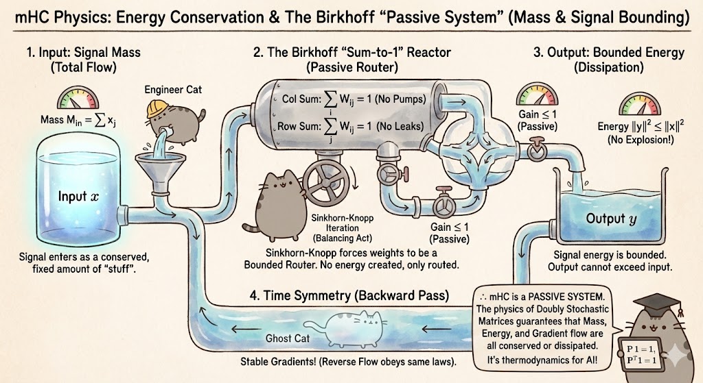
The mHC Intuition: A stable deep network should act like a Passive System. It should be a complex system of pipes and valves that routes the flow (signal) but never creates it out of thin air.
Deriving the Math from the Physics
Let’s try to design a layer strictly obeying conservation laws. We will see that the Doubly Stochastic constraint naturally falls out of these requirements.
1. Conservation of “Signal Mass” (First Moment)
Imagine the input signal $x$ is a physical fluid with a total mass. We want the total mass leaving the layer to equal the mass entering it. No leaks, no pumps.
\[\sum_{i} y_i = \sum_{j} x_j\]Substituting $y_i = \sum_j W_{ij} x_j$:
\[\sum_{i} \sum_{j} W_{ij} x_j = \sum_{j} x_j\]If we swap the summation order to isolate the input terms:
\[\sum_{j} x_j \left( \sum_{i} W_{ij} \right) = \sum_{j} x_j\]For this to hold for any input signal $x$, the term in the parentheses must be exactly 1.
\[\sum_{i} W_{ij} = 1 \quad (\forall j)\]Result: This forces the Column Sums to be 1. Physically, this ensures that every drop of “mass” from input $j$ is accounted for in the output.
2. Bounding “Signal Energy” (Second Moment)
Mass conservation isn’t enough; we need to prevent the variance (energy) from exploding. We want the system to be Dissipative—the output energy should never exceed the input energy.
\[\|y\|^2 \le \|x\|^2\]To guarantee this without complex eigenvalue analysis, we can demand that the output is a Convex Combination (a weighted average) of the inputs.
\[y_i = \sum_j W_{ij} x_j \quad \text{where } W_{ij} \ge 0\]By Jensen’s Inequality, since $\sum_j W_{ij} = 1$ (which we will enforce momentarily) and weights are non-negative:
\[(y_i)^2 = \left(\sum_j W_{ij} x_j\right)^2 \le \sum_j W_{ij} (x_j^2)\]Summing over all outputs to get total energy:
\[\|y\|^2 = \sum_i y_i^2 \le \sum_i \sum_j W_{ij} x_j^2\]Swapping sums again:
\[\|y\|^2 \le \sum_j x_j^2 \underbrace{\left( \sum_i W_{ij} \right)}_{=1} = \|x\|^2\]Result: By forcing $W$ to be non-negative and sum-to-one, we mathematically guarantee that Energy Out $\le$ Energy In. The gradient cannot explode because the system cannot amplify.
3. Time Symmetry (The Backward Pass)
Here is the final piece of the puzzle. A neural network is a bidirectional system.
- Forward Pass: Data flows through $W$.
- Backward Pass: Gradients (Error Energy) flow through $W^T$.
If we only conserve energy in the forward direction (Column Sums = 1), we might still explode during backpropagation. The “Ghost Cat” of the gradient needs a stable path too.
The total “error mass” being propagated back is:
\[\sum_{j=1}^d (g_{out})_j = \sum_{i=1}^d (g_{in})_i \underbrace{\left( \sum_{j=1}^d W_{ij} \right)}_{\text{Row Sum}}\]To ensure Gradient Energy Conservation, we must apply the same logic to $W^T$, forcing the Row Sums to be 1:
\[\sum_{j} W_{ij} = 1 \quad (\forall i)\]
Another angle: The Information Theoretic View
If Physics is about conserving energy, Information Theory is about conserving bits.
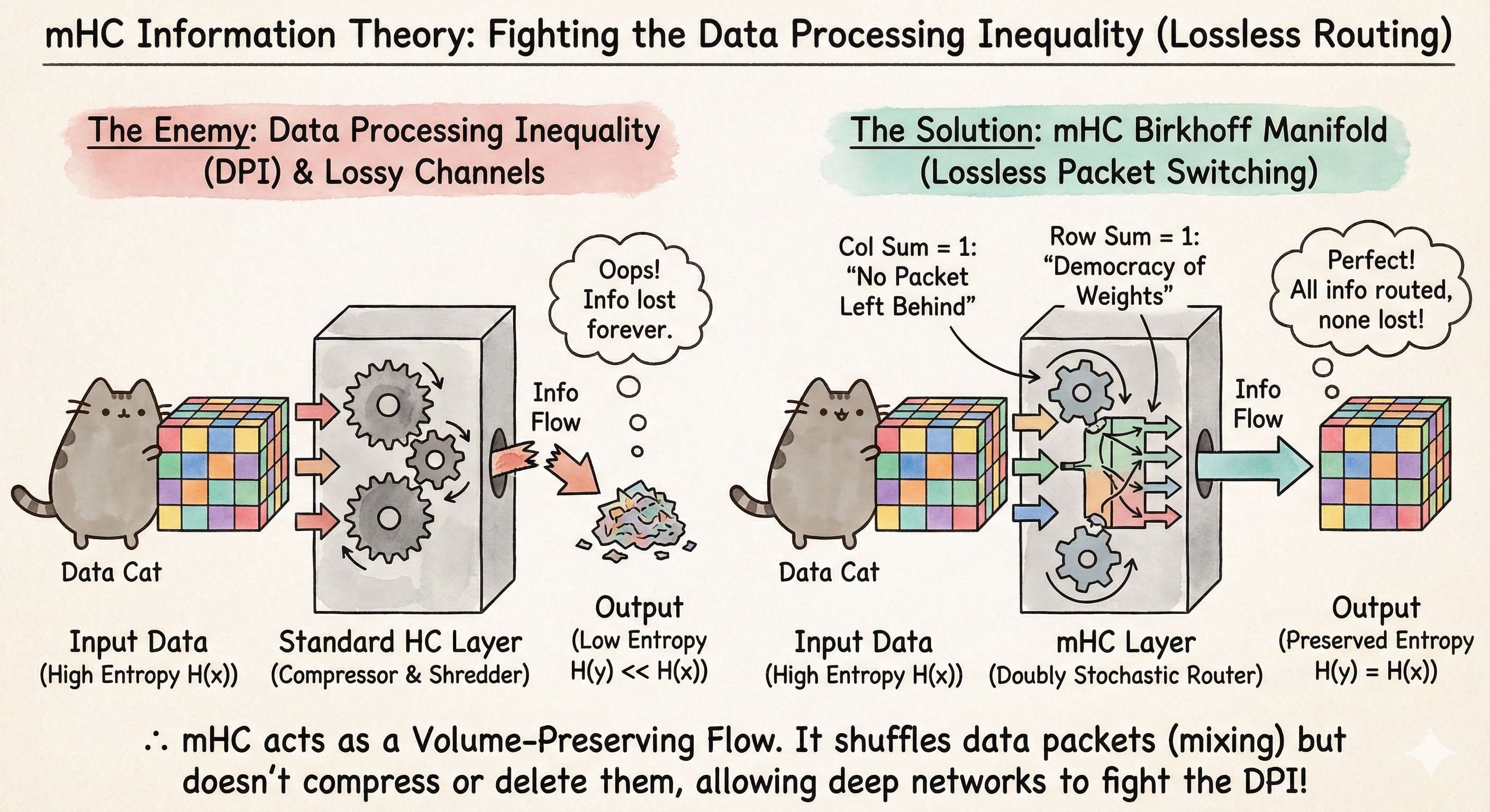
The Enemy: The Data Processing Inequality
The fundamental law of information processing is the Data Processing Inequality (DPI). It states that as you pass data $X$ through a chain of processors (layers), the Mutual Information $I(X; Y)$ can only decrease or stay the same. You cannot create information about the input deep in the network.
\[I(X; Y_{deep}) \le I(X; Y_{shallow})\]Standard layers are often Lossy Channels.
- Rank Collapse: If $W$ projects high-dimensional data into a lower-dimensional subspace, information is permanently deleted.
- Mode Collapse: If the network decides “only feature A matters” and sets weights for feature B to near-zero, feature B is lost forever.
The Solution: The Network as a “Packet Switcher”
What is the most information-efficient operation possible? A Permutation. If you simply shuffle the order of the data packets, $H(y) = H(x)$. You have preserved 100% of the information.
mHC relaxes this “Hard Permutation” into a “Soft Routing” scheme via the Birkhoff Polytope (the set of doubly stochastic matrices).
1. “No Packet Left Behind” (Column Sum = 1)
The Column Sum constraint ($\sum_i W_{ij} = 1$) is a guarantee of Signal Preservation. It dictates that 100% of the signal coming from Input Node $j$ must go somewhere. It cannot be multiplied by zero. It forces the network to find a destination for every feature.
- Info Theory Benefit: This prevents the network from ignoring subtle features early on, preserving the Channel Capacity for deeper layers.
2. “The Democracy of Weights” (Majorization)
The Row Sum constraint ($\sum_j W_{ij} = 1$) prevents Hub Neurons. No single output neuron is allowed to hoard all the connections. If a neuron wants to attend to one feature, it must ignore others.
- Info Theory Benefit: This forces the information to be “Spread Out” (Maximized Entropy). It prevents the signal from collapsing into a few “spikes” and ensures a Distributed Representation where every neuron carries a share of the information load.
By forcing the weight matrix to be Doubly Stochastic, mHC effectively turns the layer into a Volume-Preserving Flow. It allows the signal to be mixed and routed without being compressed (loss) or expanded (noise), fighting the Data Processing Inequality at every step.
The Mathematical Engine: Doubly Stochastic Matrices & Sinkhorn-Knopp
When we combine these three physical requirements:
- Mass Conservation $\rightarrow$ Column Sums $= 1$
- Dissipative Energy $\rightarrow$ Non-negative weights ($W \ge 0$)
- Time Symmetry $\rightarrow$ Row Sums $= 1$
We arrive at exactly the definition of a Doubly Stochastic Matrix.
The set of all such matrices is the Birkhoff Polytope ($\mathcal{B}_n$). The mHC paper didn’t arbitrarily choose this manifold; it is the only geometric space that satisfies these conservation laws.
The Enforcer: The Sinkhorn-Knopp Algorithm
We initialize our network with random weights $A$ that likely violate all these laws (negative values, random sums). How do we project this chaotic matrix $A$ onto the stable Birkhoff Polytope?
We use the Sinkhorn-Knopp Algorithm, an iterative “pressure equalization” process.
Step 1: Enforce Positivity (The Energy Floor) We ensure strictly positive energy transfer by taking the exponential: \(S^{(0)}_{ij} = \exp(A_{ij})\)
Step 2: Iterative Normalization We alternate between normalizing rows and columns.
-
Row Normalization (Conservation in Time): \(S^{(k)}_{ij} \leftarrow \frac{S^{(k-1)}_{ij}}{\sum_{l} S^{(k-1)}_{il}}\)
-
Column Normalization (Conservation of Mass): \(S^{(k+1)}_{ij} \leftarrow \frac{S^{(k)}_{ij}}{\sum_{l} S^{(k)}_{lj}}\)
Step 3: Convergence Sinkhorn’s Theorem guarantees that this process converges to a unique matrix $P \in \mathcal{B}_n$:
\[\lim_{k \to \infty} S^{(k)} = P \quad \text{s.t.} \quad P \mathbf{1} = \mathbf{1}, \quad P^T \mathbf{1} = \mathbf{1}\]In practice, mHC typically uses just 3-5 iterations. This forces the neural network to stop playing dice with energy and start respecting the laws of thermodynamics.
See, mHC isn’t just a constraint; it’s a statement that Stability is Symmetry.