The missing knowledge snippets of AI
It is a live blog post of some knowledge snippets of AI to bridge the gap among text books, papers, other blog posts. Most content has been posted on my Linkedin.
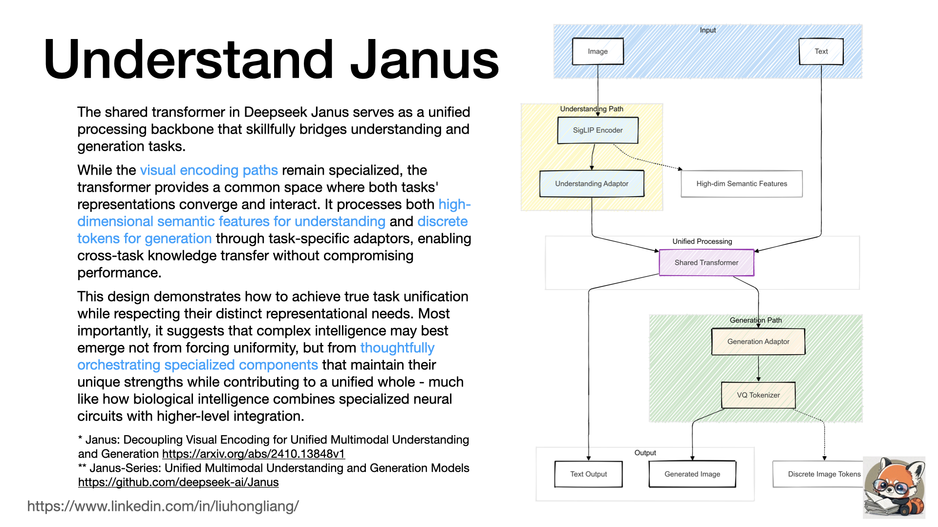
Understand Janus
The architectural design of Deepseek Janus https://github.com/deepseek-ai/Janus reflects both engineering pragmatism and cognitive science inspiration. From an engineering perspective, the dual-pathway design with a shared transformer backbone elegantly solves the tension between specialized processing needs and unified reasoning. The separate visual encoders optimize for their specific tasks - semantic understanding versus detailed reconstruction - while the shared transformer enables efficient parameter usage and cross-task learning. This architecture also aligns with Minsky’s Society of Mind theory, where intelligence emerges from the coordination of specialized agents. The visual pathways act as dedicated sensory agents with distinct expertise, while the transformer serves as a higher-level cognitive space where different representations can interact and integrate, similar to how human association cortices coordinate between sensory and linguistic processing. This parallel suggests that effective multimodal AI architectures might benefit from embracing both specialized processing and unified reasoning, mirroring the brain’s strategy of maintaining dedicated systems while enabling high-level integration.
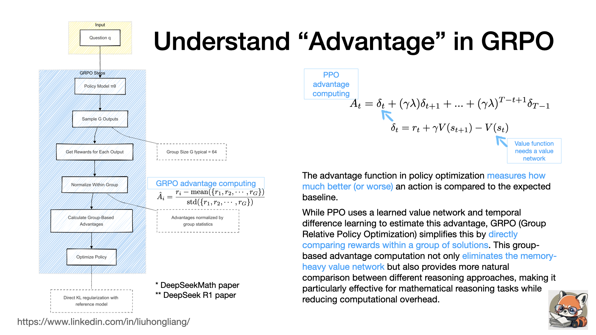
Understand Advantages in GRPO
In DeepSeek Math and R1 papers, GRPO (Group Relative Policy Optimization) introduces a fundamental redesign of advantage computation in policy optimization. While advantage traditionally measures how much better an action is compared to a baseline, the way to compute this advantage marks a key difference between GRPO and traditional PPO (Proximal Policy Optimization). Traditional PPO relies on a learned value network and temporal difference learning to estimate advantages, requiring additional memory and computation to maintain a separate critic network. In contrast, GRPO takes a more direct approach by sampling multiple solutions for the same problem and computing advantages through group statistics. This group-based normalization naturally captures the relative performance of different solutions. The impact of this design is particularly significant for mathematical reasoning tasks. By eliminating the value network, GRPO reduces memory usage by approximately half. More importantly, the group-based comparison aligns well with how mathematical solutions should be evaluated - relative to other approaches to the same problem. This makes GRPO especially effective for training models to develop better reasoning strategies, as demonstrated in both DeepSeek Math and R1’s strong performance on mathematical reasoning benchmarks, while maintaining computational efficiency and training stability.
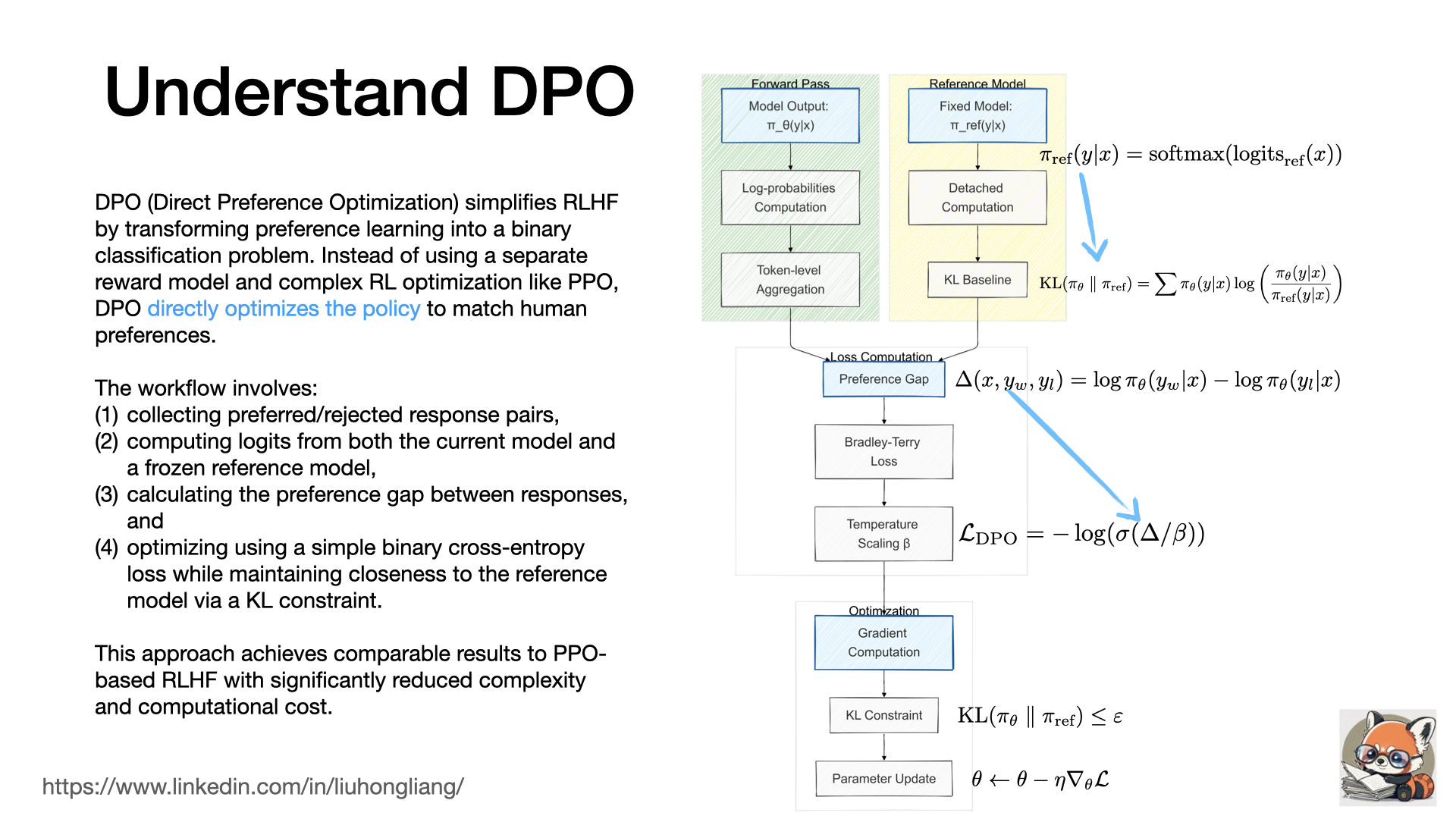
Understand Direct Preference Optimization (DPO)
DPO (Direct Preference Optimization) simplifies RLHF by transforming preference learning into a binary classification problem. Instead of using a separate reward model and complex RL optimization like PPO, DPO directly optimizes the policy to match human preferences.
The workflow involves:
- collecting preferred/rejected response pairs,
- computing logits from both the current model and a frozen reference model,
- calculating the preference gap between responses, and
- optimizing using a simple binary cross-entropy loss while maintaining closeness to the reference model via a KL constraint.
This approach achieves comparable results to PPO-based RLHF with significantly reduced complexity and computational cost.
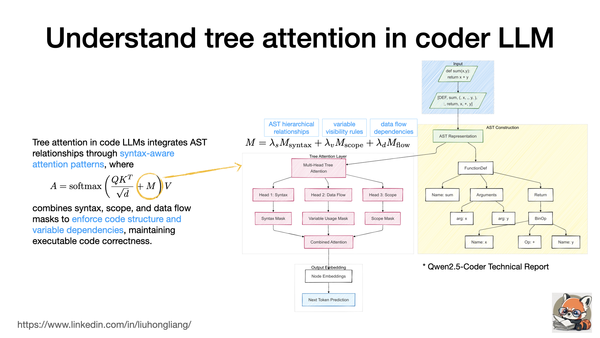
Understand tree attention in coder LLM
Tree attention in code LLMs enhances structural understanding by incorporating Abstract Syntax Tree (AST) relationships into the attention mechanism. The model learns syntax-aware attention patterns through multi-head attention where different heads specialize in parent-child relationships, variable scoping, and data flow. During training, attention scores are computed as $A = \text{softmax}\left(\frac{QK^T}{\sqrt{d}} + M\right)V$ , where $M$ combines syntax, scope, and data flow masks. These masks guide attention to respect code structure: syntax masks encode AST hierarchy, scope masks enforce variable visibility rules, and data flow masks track variable dependencies. This enables the model to maintain structural coherence even when processing linear code input. This approach is necessary because code fundamentally differs from natural language in its strict hierarchical structure and precise execution semantics. While natural language models can tolerate some structural ambiguity, code requires exact understanding of scope boundaries, variable dependencies, and control flow. Without tree attention, models struggle with long-range dependencies (like tracking variable definitions across functions), nested structures (maintaining proper code blocks), and scope rules (knowing which variables are accessible where). This affects their ability to generate syntactically valid and executable code. Tree attention solves these issues by explicitly modeling the AST structure through attention masks, enabling the model to reason about code in a way that matches how compilers and developers understand it.
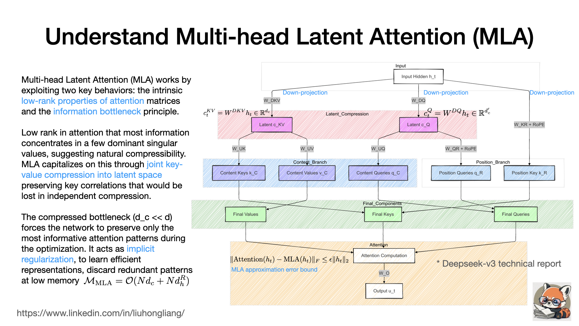
Understand Multi-head Latent Attention (MLA)
In Deepseek-v3 technical report, the team introduces Multi-head Latent Attention (MLA). MLA leverages two key insights about attention mechanisms: (1) attention matrices exhibit low-rank properties since token relationships often focus on limited patterns (local context, semantic anchors), and (2) information bottleneck can help preserve essential patterns while discarding redundant ones. The process flows as:
CopyInput h_t → [Joint KV Compression via W_DKV] → Latent c_KV
           → [Up-project] → Keys k_C and Values v_C (content)
           + [Separate RoPE branch] → Positional k_R
The joint compression ($h_t$ → $c_{KV}$) preserves crucial correlations between keys and values that would be lost in independent compression. Meanwhile, separating positional information ($k_R$) exploits the simpler structure of positional relationships. The compressed latent space (d_c ≈ d/14) creates an information bottleneck that forces the network to preserve only the most informative attention patterns during optimization, effectively acting as implicit regularization.
This design reduces memory from $\mathcal{O}(Nd_h n_h)$ to $\mathcal{O}(Nd_c + Nd^R_h)$ while maintaining model quality, as the compression preserves the dominant singular values of the attention matrix that carry the most important relationship information.
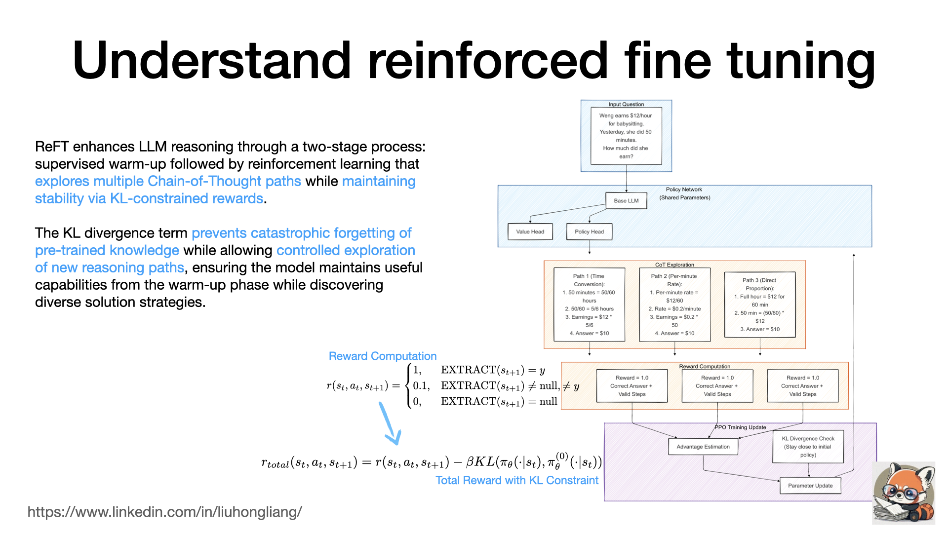
Understand Reinforced fine tuning
ReFT (Reasoning with Reinforced Fine-Tuning) https://arxiv.org/abs/2401.08967 addresses a fundamental limitation in LLM reasoning by extending beyond traditional supervised fine-tuning’s single-path learning approach. The method employs a two-stage process: an initial supervised warm-up followed by a PPO-based reinforcement learning phase that enables exploration of multiple valid reasoning paths, with a critical KL divergence constraint that prevents catastrophic forgetting of pre-trained knowledge while enabling controlled exploration. During the RL phase, the model samples various Chain-of-Thought (CoT) approaches - for example, when solving a math problem about hourly wages, it might explore different strategies like time conversion (50min to 5/6 hour), per-minute rate calculation ($ 12/60 * 50), or direct proportion ((50/60) * $ 12) - and receives rewards based on answer correctness (1 for correct, 0.1 for extractable but incorrect, 0 for invalid), while a KL divergence term (β=0.01 for P-CoT, 0.05 for N-CoT) maintains stability by preventing excessive deviation from the warm-up policy. What’s particularly remarkable is ReFT’s effectiveness with limited training data - requiring only hundreds of examples to achieve significant improvements. This efficiency stems from its ability to generate multiple learning signals from each example through active exploration of the reasoning space, creating a self-augmenting training process where each example seeds the discovery of various solution strategies while maintaining alignment with the pre-trained knowledge via KL constraints. ReFT maximizes learning from each example by exploring multiple reasoning paths while using the KL divergence to maintain useful pre-trained knowledge, effectively creating a self-augmenting training process that generates diverse learning signals from limited examples. The method’s success stems from its ability to learn from both successful and unsuccessful reasoning attempts, combined with a natural reward structure that eliminates the need for a separate reward model. When integrated with inference-time techniques like majority voting and reward model reranking, ReFT demonstrates even more impressive results.
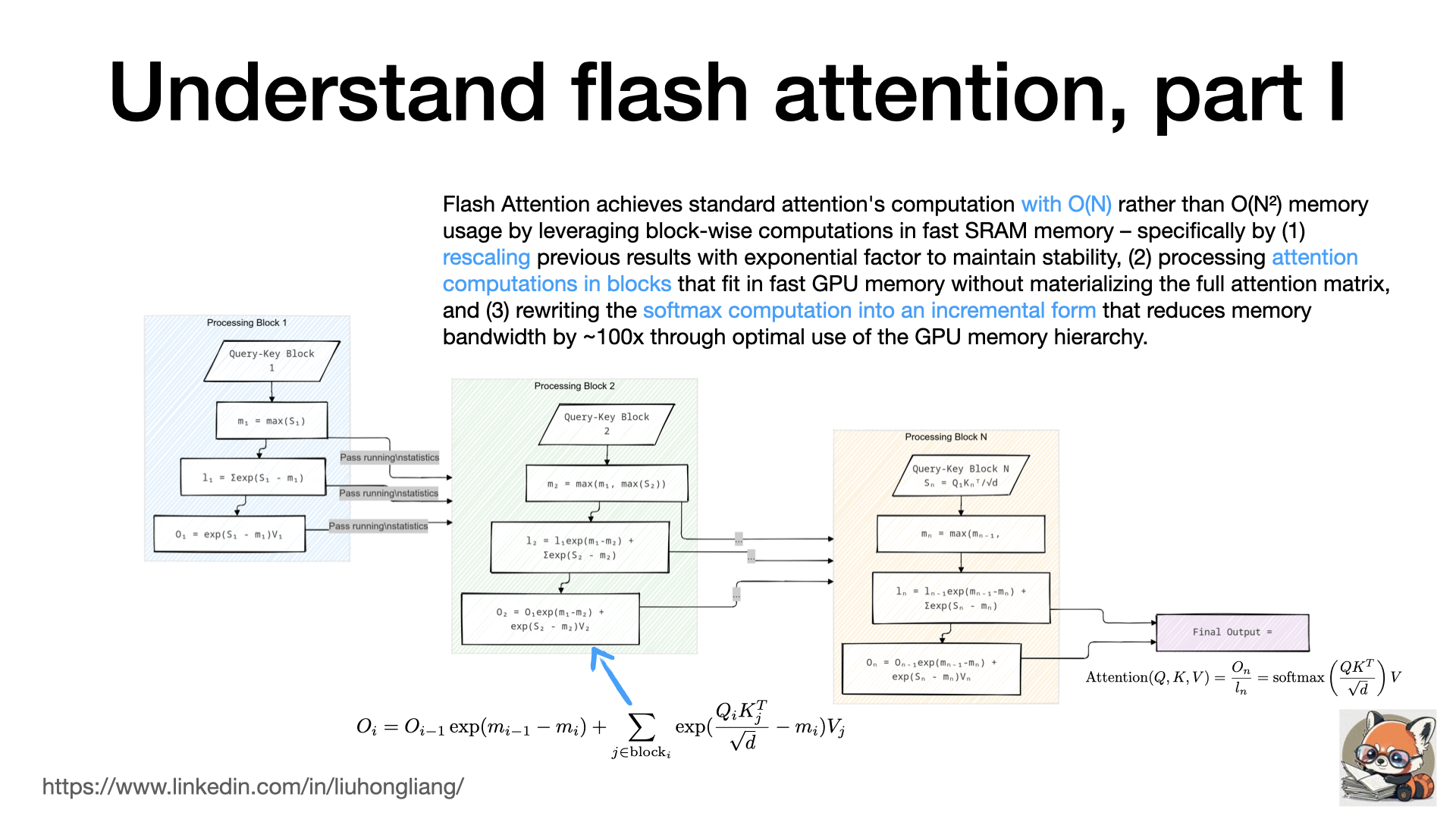
Understand Flash Attention, incremental computation of attention
Flash Attention’s incremental computation is a mathematically elegant solution to the memory bottleneck in attention mechanisms. The key insight is treating attention computation as a streaming algorithm with running statistics. Instead of materializing the full N×N attention matrix, it maintains three running statistics: maximum values \(m_i\) for numerical stability, softmax denominators \(l_i\), and partial output sums \(O_i\). When processing each new block, these statistics are updated using a clever rescaling factor \(\exp(m_{i-1} - m_i)\) that ensures mathematical equivalence to standard attention while preventing numerical overflow. This rescaling is crucial because it allows us to update our running computations when we discover new maximum values in later blocks - effectively “correcting” our previous partial results without needing to store or recompute them. The computation is structured as a tiled algorithm where blocks of queries interact with blocks of keys and values, with all intermediate results fitting in fast SRAM. This approach reduces memory complexity from \(\mathcal{O}(N^2)\) to \(\mathcal{O}(N)\) and significantly improves hardware utilization by maximizing the use of fast memory (SRAM) over slow memory (HBM), resulting in both better memory efficiency and faster computation. The mathematical guarantee of equivalence to standard attention, combined with these performance benefits, makes it particularly valuable for training and deploying large language models where attention computations are a major bottleneck.
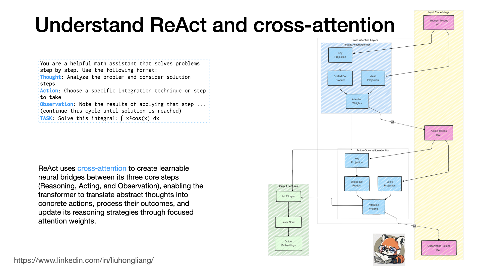
Understand ReAct and cross-attention
How could ReAct agents be effective on reasoning and acting? What was behind “Thought Action Observation”?
ReAct was one of the important LLM agent techniques https://lnkd.in/gU4jB6FA and ReAct’s effectiveness comes from its three major steps (Reasoning, Acting, and Observation) being tightly coupled through cross-attention mechanisms. The Reasoning step generates abstract thought representations in the transformer’s embedding space, where self-attention helps form coherent reasoning chains. These thought embeddings then flow into cross-attention layers that map them to concrete action embeddings, effectively translating abstract reasoning into executable actions. The Action step’s outputs generate observations, which are processed through another set of cross-attention layers that integrate these results back into the model’s understanding.
The key to ReAct’s effectiveness lies in how cross-attention serves as neural bridges between these steps: it creates learnable mappings between abstract thought space and concrete action space (Thought→Action), between actions and their outcomes (Action→Observation), and between observations and updated reasoning (Observation→Thought). This creates a continuous feedback loop where each step informs the next through focused attention weights, allowing the model to learn from experience and adapt its strategies. The cross-attention mechanisms also enable the model to maintain relevant context throughout the entire process, as attention weights highlight important information from previous steps while suppressing irrelevant details. This architecture naturally implements a form of working memory and metacognition, where the model can reflect on its own reasoning and actions through the attention patterns, leading to more effective problem-solving strategies. It is one of the effective ways to extend the LLM runtime for more “smartness”.
Understand constrained decoder and JSON mode
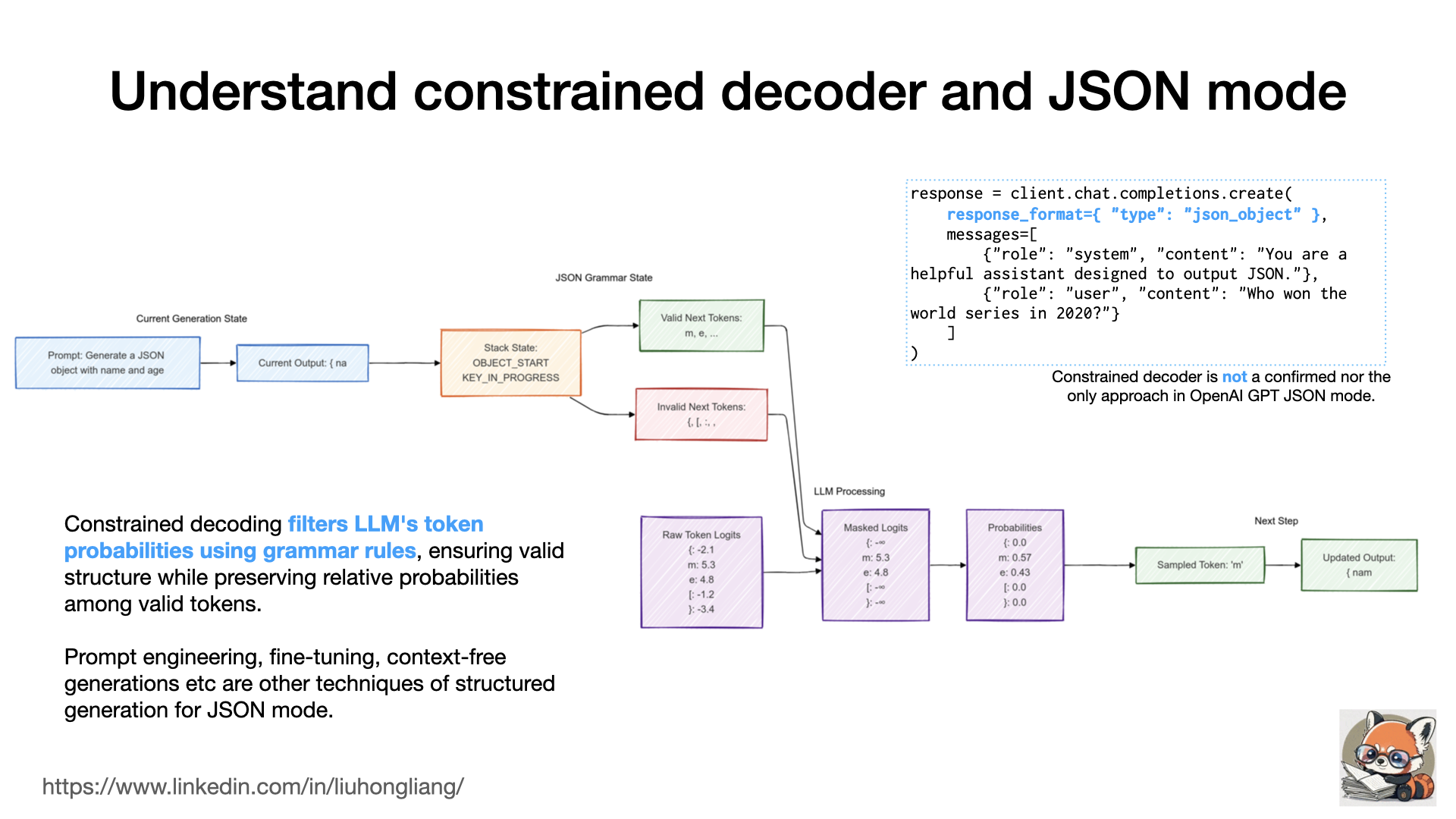
How did GPT guarantee a JSON output in its JSON mode? How was it implemented in other solutions like .txt and XGrammar?
One of the key techniques was called constrained decoding. It bridges neural language models with formal grammar constraints by modifying the model’s output distribution during generation. At each autoregressive step, instead of directly sampling from the LLM’s logits across its vocabulary (e.g., 128k tokens for Llama 3), the approach applies a mask derived from a context-free grammar (CFG) to ensure structural validity. Technically, this is implemented by setting logits of invalid tokens to -∞ before the softmax operation, effectively zeroing their sampling probabilities while preserving the relative probabilities among valid tokens. The grammar state is tracked using a pushdown automaton (PDA) that maintains a stack for nested structures. Modern implementations like XGrammar https://lnkd.in/gVyHKhp3 optimize this process by classifying tokens into context-independent ones (validity determined by current state only) and context-dependent ones (requiring full stack context), enabling efficient preprocessing and caching.
Surely, neither constrained decoding nor context-free generation could be the only approach of JSON mode. Meanwhile, structured generation is a superset research field of JSON generation for other structures. Structured generation is a corner stone for the agent framework, so that agents can communicate and understand in the JSON way.
Understand RoPE and lost-in-the-middle
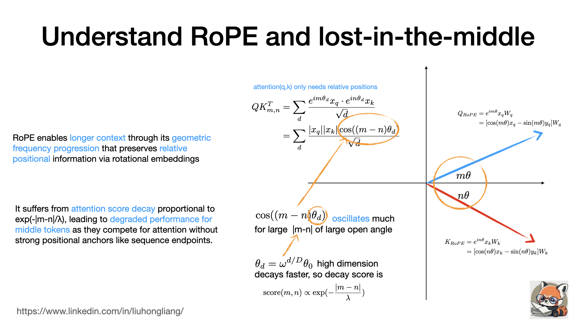
Why LLM could get long context using Rotary Positional Embedding (RoPE)? but why “lost-in-the-middle” came with it?
Rotary Positional Embedding (RoPE) is a simple and great idea: attention is about dot products of vectors, why don’t we just use the polar coordinate in multiple dimensions? In RoPE, attention computing only depends on relative positions, a.k.a summation of cosine of two vectors in each dimension, so any context can rotate and stack up where the attention is preserved. But the problem comes after it: cosine function oscillates much when |m-n| becomes large, without a good starting point, the relative position just gets lost. The higher dimension in the embedding, the worse attention decay.
Let’s think of RoPE like a spiral staircase in a tall tower: as you go higher (higher dimensions), you rotate faster, but the fundamental structure (relative positions) stays consistent. This allows you to keep track of where you are relative to other positions, even in a very tall tower (long context). And the “lost-in-the-middle” problem is like trying to remember specific floors in the middle of the tower: you easily remember the ground floor (start) and top floor (end), but floors in the middle blur together because they lack these distinctive reference points and each middle floor looks similar to its neighbors.
Understand speculative decoding
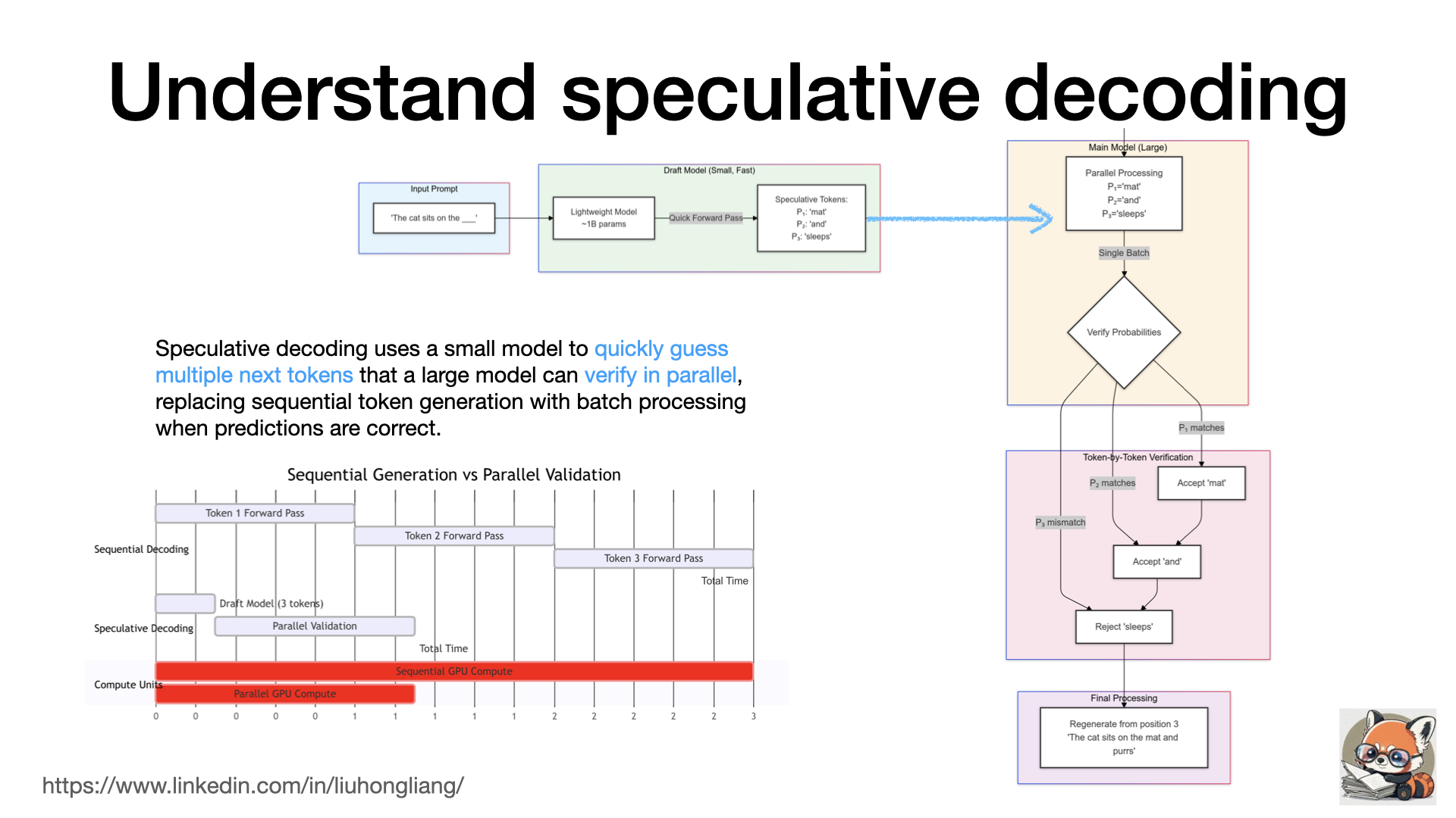
What is “speculative decoding”? why it could speed up LLM generation?
In my last post of LLM inference time https://lnkd.in/gu78UWtH I mentioned a few alternatives to “next token generation” in sequence, and speculative decoding is one of them. It accelerates LLM inference by using a small, fast “draft” model to predict multiple tokens ahead, e.g. “mat” “and” “sleep” for “The cat sits on the ___”, while letting the main model verify these predictions in parallel through a single forward pass, accepting correct predictions and falling back only when necessary - essentially trading some extra compute from a lightweight model to reduce the number of expensive forward passes in the large model.
Such process reminds us of the modern CPU’s branch predictor: when a CPU see an “if” statement, it tries to guess which way a branch will go before knowing the results, so the instruction flow can move very fast without much waiting time. Speculative decoding shortens the total execute time by replacing N times of forward pass time with a round of draft plus a single forward pass time.
Understand LLM inference time
From the first input token to the last output token, what exact happened in the LLM and why it took so long?
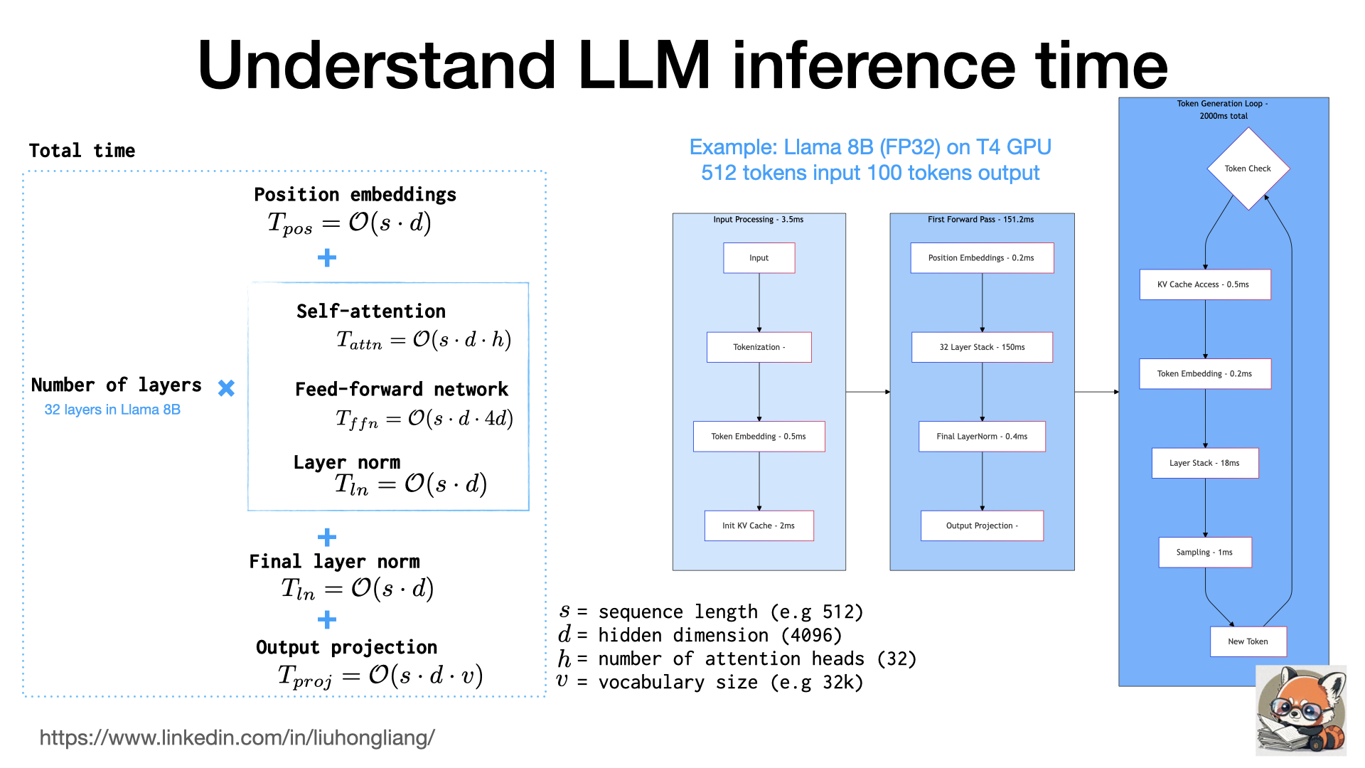
The total inference time can break down as the following:
Total time = Position embeddings + Number of layers × (Self-attention computation + Feed-forward network computation + Layer norm operations) + Final layer norm + Output projection
where self-attention and FFN took mostly of the computing time, and we had to do it 32 times if a LLM like llama 8B had 32 layers. That also explained why LLM has significant different input and output speed: the input sequence just fed in and went through all 32 layers once (and warmed up KV cache), while each output token one-by-one went through the token generation loop, went through all 32 layers, put back to the sequence due to self-aggregation, and added next token. There was some research work on advanced token generation instead of one-by-one output.
We could also understand the quantization effect to speed up: attention and FFN took the most computing time, and total time was mostly proportional to number of generated tokens. If we used FP16 instead of FP32, attention and FFN could cut the computing time to half, and the total computing time could reduce ~40% (well, layer norm time didn’t change much in precision). If used INT8, we could further reduce another 30% but increased the risk of precision loss.
Understand LoRA ranks
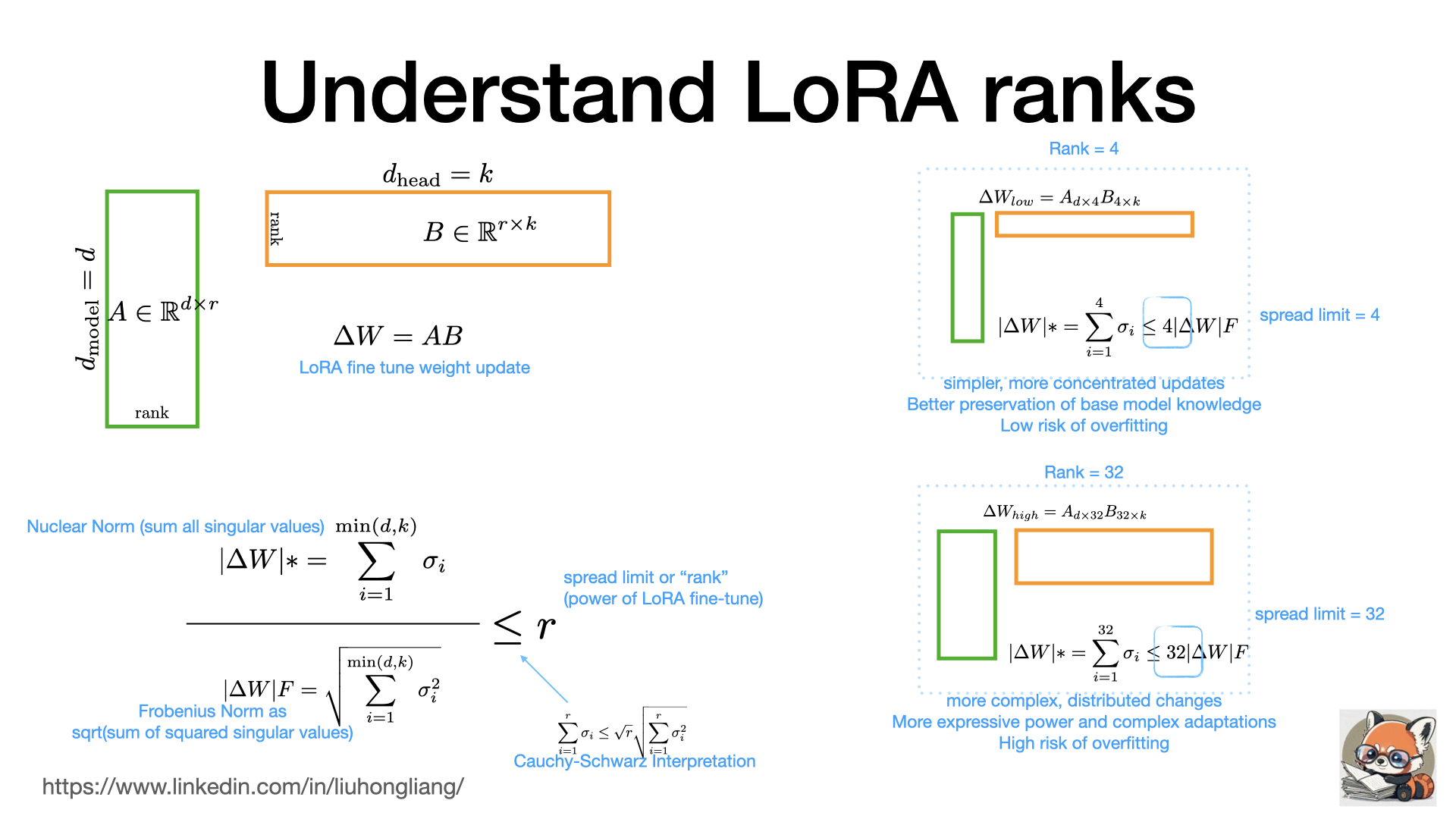
Why rank matters in LoRA fine tune? why more knowledge adoption always comes with risk of overfitting in my LLM?
We love LoRA for its efficiency and low memory cost. We know LoRA fine tune is a decomposition of the update of weight matrix. Lower rank gives thinner matrix A and B. For example, if LoRA tune in attention layers, low rank only modifies a few attention patterns simultaneously, less likely to break existing patterns and less likely to disrupt critical cross-attention mechanisms. We usually follow the following rule of thumbs:
Knowledge injection: lower ranks (4-8) often sufficient Domain adaptation: medium ranks (16-32) usually better Complex reasoning changes: might need higher ranks (64+)
To understand the effect, consider each row in the matrix means update to a dimension, and the ratio of nuclear norm of the matrix vs forbenius norm means how much the information can spread in how many dimensions in the singularity matrix. The upper limit of the information spread is the rank. It explains much about the fine tune effect: low rank spread new knowledge toward the first a few dimensions and high rank can update in more dimensions, where new knowledge has deeper reach but brings in more risk of overfitting. Surely it is the upper limit of information spread, and it doesn’t promise the new information can reach that far.
You might wonder why it is “less or equal” instead of “equal”. It is because of Cauchy–Schwarz inequality for vectors https://lnkd.in/gKmjMKK6 which can also describe proper time measurement in relativity, a.k.a “you move fast your clock is slower”. There is always physics!
Understand chain-of-thoughts (CoT)
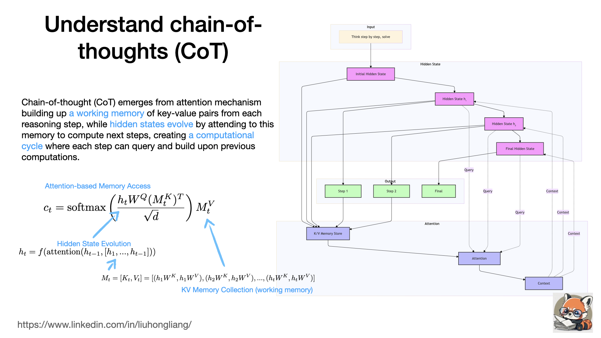
Why LLM could do chain-of-thought? what exactly happened when LLM received a “think step by step” instruction?
CoT practically uses attention as working memory for each reasoning step for a computing cycle to evolve the hidden states in the neural network. When each new hidden state from a later reasoning step could query and update from the previous memory, it leads to a “step-by-step” reasoning. The key is about memory from the previous states!
It helps us to understand why sometimes CoT works well sometimes not: if a problem only needs its previous state and a piece of memory, CoT works well, otherwise, we need more complex reasoning models like OpenAI o1, since human can keep a long memory with branches and try-errors. Don’t forget human can also think P and ~P!
It also gives a good hint of memory package design if we want to extend such memory mechanism with longer or external memory.
Understand tool using
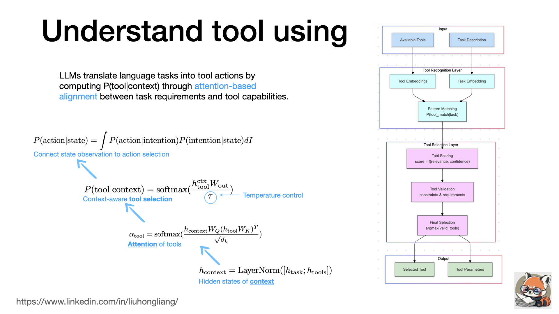
What is the magic behind LLM’s tool using, like Apple Intelligence? a.k.a how come some language models can understand and call an API and some not?
Tool using, like “function calling” in OpenAI https://lnkd.in/gjMwbmaM , opens a door to drive intelligent agents from LLM. Beyond just letting LLM generate a JSON to call an API, it is trained and tuned by aligning tasks with tool capabilities using attention of context and tools. When we use such functionalities, the LLM simply maximize the conditional probability of current context vs a tool by comparing context with tool description. That is the root reason why one must describe a tool in a concise and accurate way in any tool calling interface. We also understand tool calling doesn’t need large models, since it only needs attention alignment with tools, so small on-device LLMs like Phi3 or Llama 3.2 1b can do tool calling well if instruct trained well. Yes, it is part of Apple Intelligence LLM’s secret recipe.
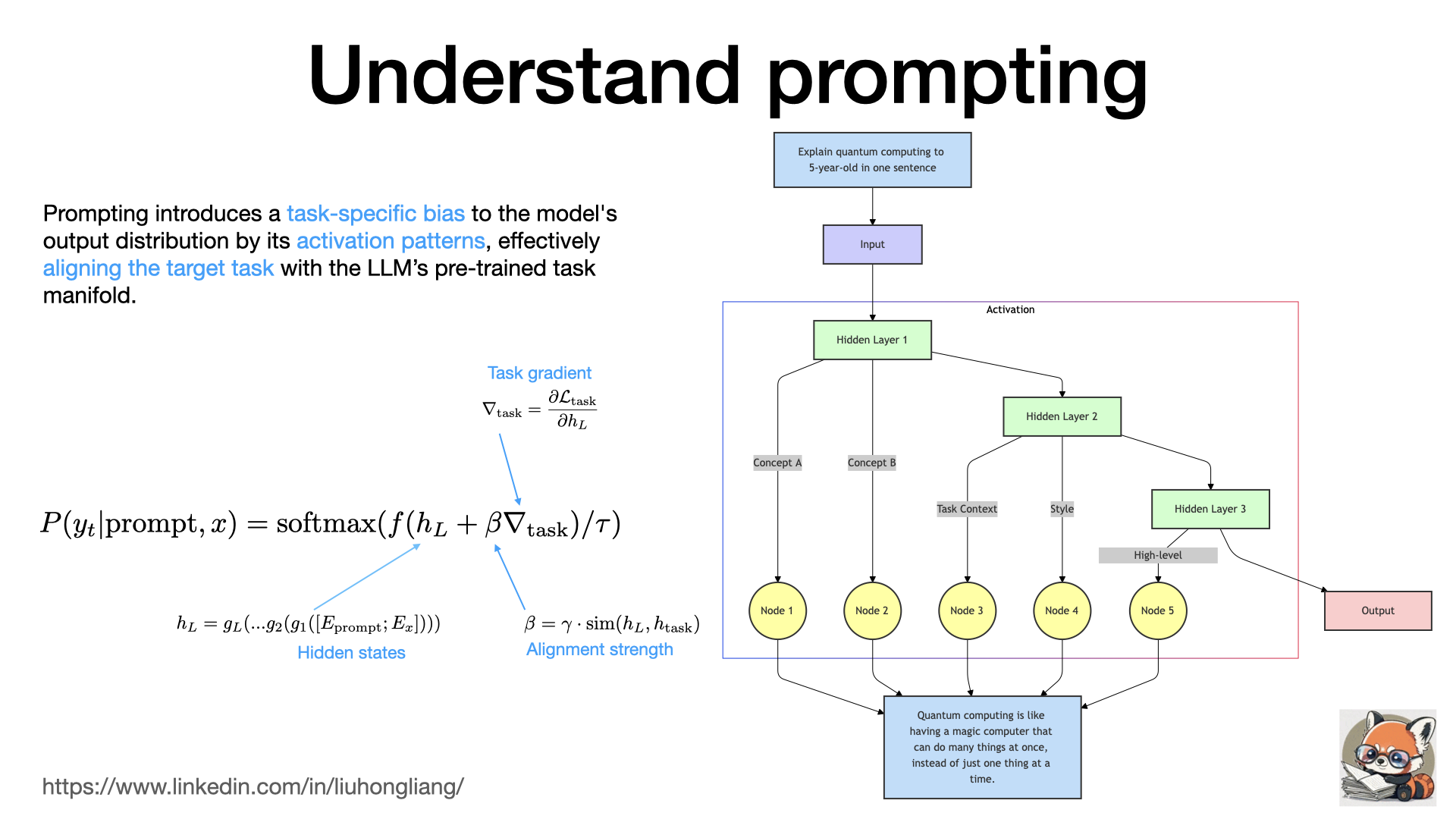
Understand prompting
What exactly happened when LLM received a prompt, why “prompting” can magically work.
Most “prompting” work today is about discrete prompt, e.g. a sentence of command. Prompting introduces a task-specific bias to the model’s output distribution by its activation patterns, effectively aligning the target task with the LLM’s pre-trained task manifold. With this short definition, we can easily understand that prompts don’t change LLM, instead, they activate certain parts of the LLM neural network by breaking down the target task and aligning it with the similar trained tasks inside LLM. That is also why LLM can’t really “reason” but simulate the reasoning process if part of the process was trained in some familiar ways. Smaller tasks with agents usually work better than a long complex prompt because LLM could align small and simple tasks easier, so we either define our task process or let another agent breakdown the complex tasks.
In short, prompting is about putting bias to models and alignment to tasks.
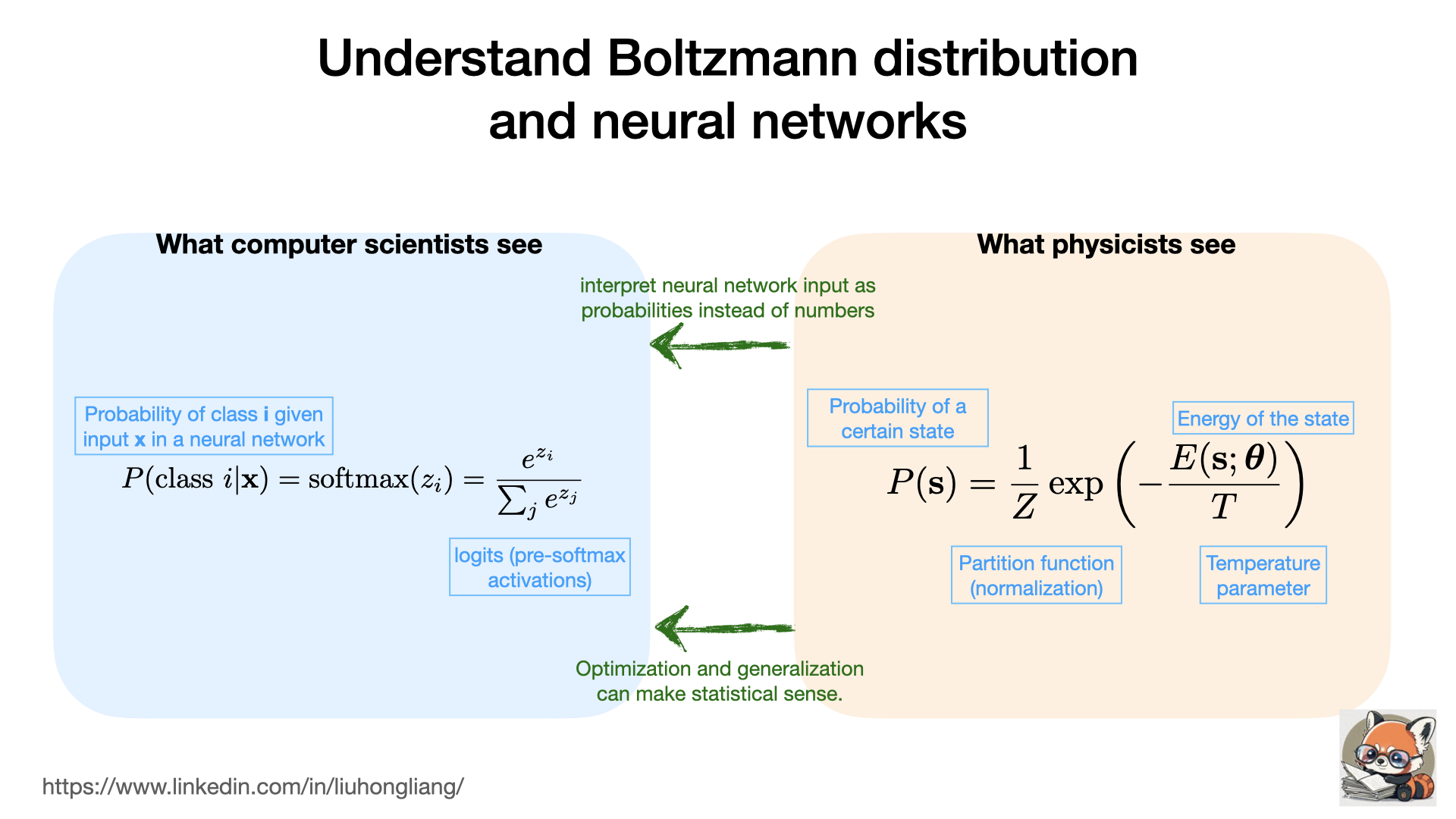
Understand Boltzmann distribution and neural networks
What exactly Geoffrey Hinton brought to neural network and AI? Statistical meanings of neural networks!
Hinton and other researchers bridged the gap between statistical physics and neural networks by interpreting neural network input as probabilities instead of numbers, so that optimization and generalization of neural networks can make sense from Boltzmann distribution. Such energy-based models were the reason why gradient decent on log(P) and why “temperature” parameter is used to control your LLM creativity. Read further at Wikipedia https://lnkd.in/geDtyTFK and congratulate that John Hopfield and Geoffrey Hinton win Nobel Prize in physics!
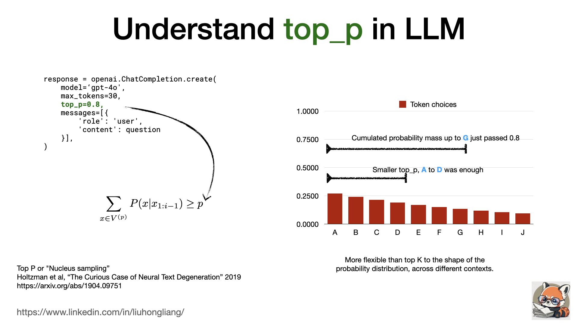
Understand top_p in LLM
What does “top P” in LLM model mean?
For a quick follow up from last post to understand high/low temperature in LLM (link https://lnkd.in/gcMDpSj4 ): why “top_p” can also control the next token choice?
Top P is the threshold of cumulated probability mass from token A to token X. For a given probability distribution, a higher top p value allows more long tail tokens. It gives more flexibility than a simple top K threshold for different context and different shape of the token probability distribution. For most cases, the combination of temperature and top_p setting can be good enough to control a LLM behavior.
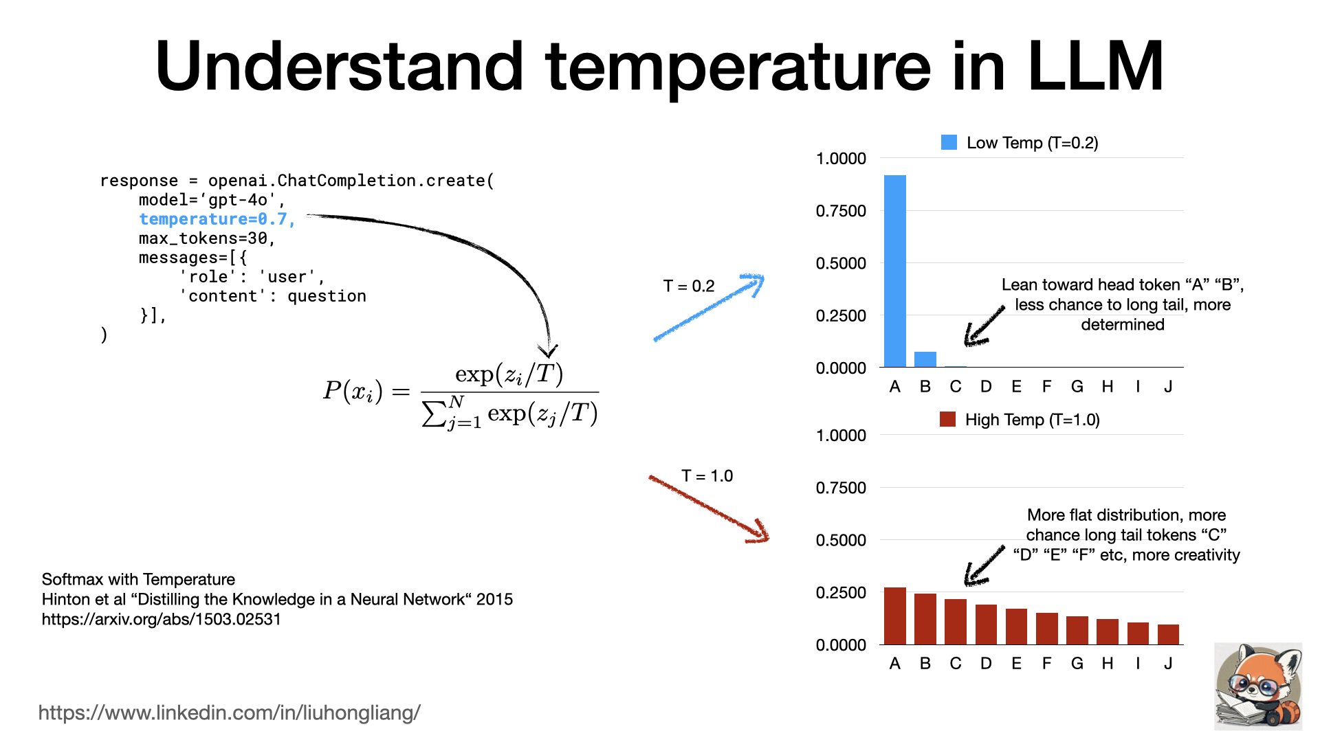
Understand temperature in LLM
What does “temperature” in LLM model mean?
Some friends recently asked me the question, why high temperature gives more creative results but much risk of hallucinations? why low temperature leads to dumb results? How to understand this magic parameter and how to use it?
Here it is one single picture to understand it: it is the “T” from softmax with temperature from Hinton et al “Distilling the Knowledge in a Neural Network“ https://lnkd.in/ghCdXgWx With top-k/top-p token selection for LLM’s next token prediction, higher temperature gives more “flat” probability distribution so long tail tokens have better chance to be chosen, thus more creativity. It is the root cause of these high-low temperature behaviors.
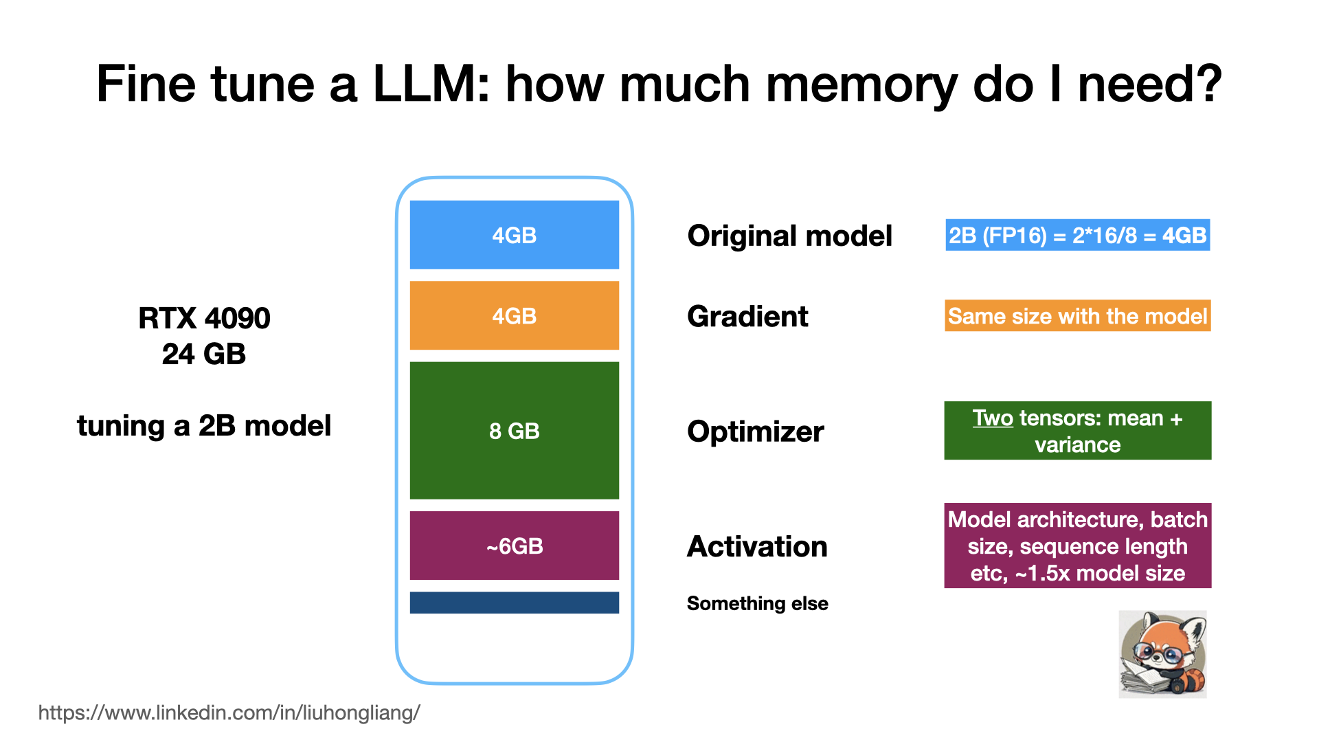
Fine tune a LLM: how much memory do I need?
Assume you bought a RTX 4090 to play “Black Myth: Wukong” and you also wanted to use it for fine-tuning a LLM. But can your gaming power handle the task?
Let’s break it down: 🧠 Model: 2B parameters, FP16 🎮 RTX 4090: 24GB VRAM
Memory cost:
- Model weights: 4GB
- Gradients: 4GB
- Optimizer states: 8GB
- Activations: ~6GB Total: ~22GB
Good news! Your RTX 4090 can handle this with just a little bit room to spare. You could even bump up the model size or batch size for better performance.
Remember, actual usage may vary based on specific architectures and frameworks. But this gives you a solid starting point for understanding LLM fine-tuning memory requirements.
Surely, there are other ways like LoRa or QLoRA of Parameter-Efficient Fine-Tuning (PEFT), along with some drawback and limits. Let’s talk about it next time.
